Maxima and Minima

This set is a disk centered at (a, b) of radius r. The primary result that is used to locate critical points of the function f is the following

Theorem
If f has a local maximum or minimum at (a, b) and f is differentiable (i.e.,for example, the first-order partial derivatives are continuous at (a, b)), then f_x(a, b) = f_y(a, b) = 0.

This implies that if f has a local maximum or minimum at (a, b) then . This imples that the normal vector of the tangent plan at the point (a, b) is <0, 0, -1>. That is the vector is parallel to the z-axis and so the tangent plane is parallel to the xy-plane.

Example f(x, y) = (x – 2y²)² + (1 – x)².

The gradient of this function is given by

Setting equal to <0, 0> we have 4x – 4y² – 2 = 0 and 8y (2y² – x ) = 0. Thus 2y² – x = 0 and so x = 2y². Substituting this into the first equation gives 8y² – 4y² = 2. Thus and so x = 1.
Thus two of the critical points are (1, 1/ ) and (1, –1/ ). Also setting y = 0 gives x = 1/2 and so the other critical point is (1/2, 0). We now have to decide which is a minimum, maximum, or neither. We see from the graph below that (1, 1/ ) and (1, –1/) are local minima and (1/2, 0) is a saddle point.

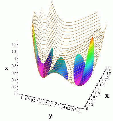
We see here that we need to determine the "concavity" of f(x, y) that is if it looks like one of the three surfaces shown below, (at least locally near the critical point).

Recall for a function of one variable g(x) with a critical point x = a, (g'(a) = 0) we know that if g''(a) > 0 then (a, g(a)) is a local minimum and if g''(a) < 0 then (a, g(a)) is a local maximum. This is shown by using a second degree Taylor polynomial approximation to g at the point a.

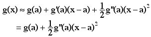
Note then that if g''(a) > 0 then g(x) "e g(a), and so (a, g(a)) is a local minimum and if g''(a) < 0 then g(x) "d g(a), and so (a, g(a)) is a local maximum.

In order to extend this to functions of more than one variable we need second degree Taylor polynomial approximation to f(x, y) at (a, b). This approximation is given by

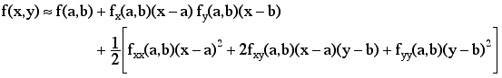
What is necessary now is how to decide when the quadratic term, (in brackets) is positive or negative for (x, y) near (a, b). This quadratic term can be rewritten using vector/matix products as:

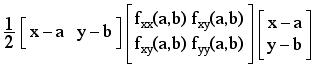
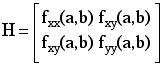
The matrix of second partial derivatives is know as the Hessian.

More generally we need to determine with a symmetric n by n matrix A is positive (negative) definite, i.e., when for all x ⁿ the quadratic form x^TA x is positive (negative). Since A is symmetric then all of its eigenvalues are real and so it can be proven that A is positive (negative) definite if and only if all of its eigenvalues are positive (negative). Recall that λ is an eigenvalue of A provided there is a nonzero vector v such that Av = λv. These eigenvalues are the roots of the characteristic polynomial det(λI – A). We state now the theorem that tells how to determine a maximum or minimum of a function of two or more variables.

Theorem Suppose u is a point in ⁿ where f = 0. Then

• f(u) is a local minimum if the Hessian matrix H at u is positive definite, i.e. the eigenvalues of H are all positive.
• f(u) is a local maximum if the Hessian matrix H at u is negative definite, i.e. the eigenvalues of H are all negative.
• If the Hessian matrix H at u is indefinite, i.e., the H has both positive and negative eigenvalues then f(u) is neither a maximum nor a minimum.

Theorem Suppose (a,b) is a point where f_x(a,b)= f_y(a,b)=0 and set D=f_xx(a,b) f_yy(a,b) – (f_xy(a,b)) ² i.e. the determinant of the Hessian matrix.

• If D > 0 and f_xx(a,b) > 0, then f(a,b) is a local minimum.
• If D > 0 and f_xx(a,b) < 0, then f(a,b) is a local maximum.
• If D < 0, then f(a,b) is a saddle, i.e., f(a,b) is neither a maximum nor a minimum.
• If D = 0, then f(a,b) could be a local minimum, local maximum, a saddle, or none of these.

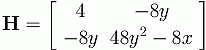
The determinant of H is given by D = 128y² – 32x. Note that f_xx(x,y) = 4 > 0, so

At (1/2, 0): D = -16 and so f(1/2,0) = 1/2 is a saddle.

At (1, 1/): D = 32 and so f(1,1/) = 0 is a local minimum.

At (1, –1/): D = 32 and so f(1,–1/) = 0 is also a local minimum.

For the situation when D = 0 consider the function f(x,y) = y³ – 4y. This function has critical points at y = 2/ and at y = –2/. The hessian matrix is given by

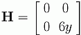
We see that the determinant of H is zero, but one of the critical points is a local maximum and the other is a local minimum. Notice the the function has a local maximum and local minimum along lines parallel to the x-axis. See the figure below.