Fourier's Approach to Heat Flow 

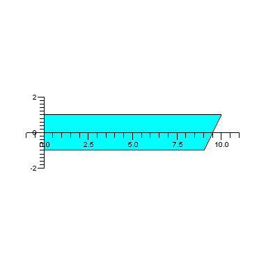
Consider the infinite rectangular lamina, 2 units wide. 

The equation that models heat flow in this lamina is given by 

Fourier was interested in the equilibrium solution where and chose the boundary conditions: 

and  As well as bounded as . 

He assumed that Substituting this into the equation gives  

Since we can separate this equation into two functions one in x only and one in y only it must be the 

case that 

a constant. 

This gives two separate equations:  

bounded

We solve the equation for G first.  We have .  Using the boundary conditions 

we have  

and  

For arbitrary values of  λ this system will have only the trivial solution and we want a nontrivial solution.  Adding these 

equations gives: .  If we take or λ.  Since  

does not satisfy the boundary conditions we take   We obtain then an infinite number of solutions given by 

For the equation we have  If we require that be 

bounded then and so  Therefore we obtain the solutions 

This then gives the equilibrium solutions as 

Fourier then noted that, the principle of superposition, that the general solution has the form 

and from the boundary condition we have to choose the values to satisfy 

(A) 

Fourier differentiated this expression and infinite number of times and generated a system for the infinite number of unknowns 

.  He offered no justification why term-by-term differentiation was possible.  Later on he noted the orthogonality of the functions 

on the interval [-1, 1]. i.e. 

Fourier then multiplies (A) by and integrates term-by-term, again with no justification.   

Note that the only nonzero term is when and we arrive at 

The solution is then given by the infinite series 

Let's consider partial sums of this function. 

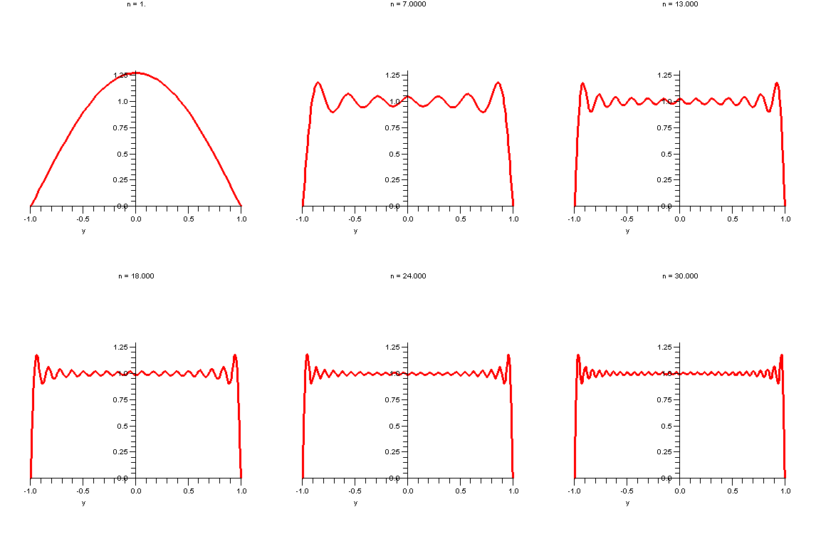
Graphs of this function for and various values of are shown below. 

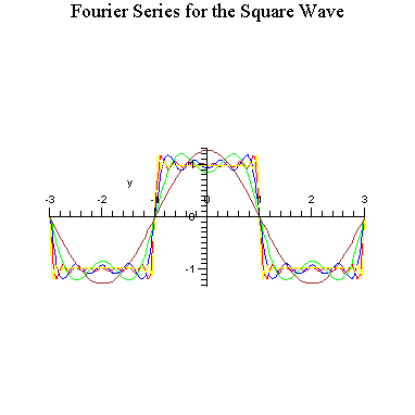
How do these partial sums converge to the square wave. 

Notice that it overshoots near the enpoints of the interval.  This is known and the Gibbs-Wilbraham phenomenom. 

For a three dimensional veiw of the solution we plot the temperature variation on the rectangle [0, 2]×[-1,1]. 

Also