SPSS On-Line Training Workshop

SPSS On-Line Training Workshop |
|
|
 In this Tutorial: |
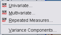
Click on the following movie clips to learn these three techniques:
Back to Statistical Procedures
|
In this on-line workshop, you will find many movie clips. Each movie clip will demonstrate some specific usage of SPSS.
Univiarate GLM is a technique to conduct Analysis of Variance for experiments with two or more factors. The main dialog box asks for Dependent Variable (response), Fixed Effect Factors, Random Effect Factors, Covariates (continuous scale), and WLS (Weighted Least Square) weight. The sub-menus include:
Model- This is the dialog for creating your model. The default is a full factorial. You can customize this to only include the interactions that you want. Sum of Squares is also set here. If there are no missing cells, Type III is most commonly used. If you have missing cells, you must use Type IV. | |
Contrasts- These are used to test for differences among the levels of a factor. They are like Post Hoc, but are specified prior to the experiment. | |
Plots- This is chosen if you want a profile (line) plot of the marginal means. | |
Post Hoc- Here you can choose multiple comparison procedures test for pair-wise comparison of group means between each pair of factor levels. Tukey's technique is generally used if you have a large number of comparisons. For a small number of comparisons, Bonferroni can also be used. | |
Save- If you want to save any of your output variables, (i.e. predicted values, residuals, diagnostics), you must choose this. You can save these to your data editor window or save them to a new file. | |
Options- Options let you select the factors for estimates of marginal means. We can also choose additional tests here (such as the Homogeneity test to confirm the assumption of equal variance) and set the significance level. |
The data set used for demonstrating the univariate GLM is the Supermarket data set. See Data Set page for details.
![]() click
here to watch Univariate ANOVA
click
here to watch Univariate ANOVA
Multivariate GLM is a technique to conduct Analysis of Variance for experiments having more than one dependent variable. This procedure can also be used for multivariate regression analysis with more than one dependent variable. The main dialog box asks for Dependent Variables (responses), Fixed Effect Factors, Random Effect Factors, Covariates (continuous scale), and WLS (Weighted Least Square) weight. The sub-menus include:
Model- This is the dialog box for creating your model. The default is a full factorial. You can customize this to only include the interactions that you want. You may want to customize if you want covariate interaction included, as this is not included in the full factorial. Sum of Squares is also set here. If there are no missing cells, Type III is most commonly used. If you have missing cells, you must use Type IV. | |
Contrasts- These are used to test for differences among the levels of a factor. They are like Post Hoc, but are specified prior to the experiment. This is only used if you have data with more than two levels. | |
Plots- This is chosen if you want a profile (line) plot of the marginal means. | |
Post Hoc- Here you can choose a test and use it to determine which means differ. Tukey is generally used if you have a large number of comparisons. For a small number of comparisons, Bonferroni can also be used. This is only used if you have more than two levels for the variable. | |
Save- If you want to save any of your output variables (i.e. predicted values, residuals, diagnostics), you must choose this. You can save these to your data editor window or save them to a new file. | |
Options- Options let you select the factors for estimates of marginal means. You can also choose additional tests here (such as the Homogeneity test to confirm the assumption of equal variance) and set the significance level. |
The data set used for demonstrating Multivariate GLM is the Plastics data set. There are 3 dependent variables; tear resistance, gloss and opacity, and two factors; extrusion and additive amount, where each factor has two levels. See the Data Set page for details.
![]() click
here to watch Multivariate ANOVA
click
here to watch Multivariate ANOVA
This technique is used to analyze a response variable which is measured at different times on the same subject. Data from repeated measures involve both 'within-subjects' factors and 'between-subjects' factors. The first dialog box asks for the information of 'within-subjects' factor name, number of levels and measure name, then, click on Define takes you to the dialog box for defining 'within-subjects' variables, 'between-subjects' factors and covariates along with the following sub-menus:
Model- This is the dialog box for defining the model, both within-subjects and between-subjects. The default is a full factorial. You can customize this to only include the interactions that you want. Sum of Squares is also set here. If there are no missing cells, Type III is most commonly used. If you have missing cells, you must use Type IV. | |
Contrasts- These are used to test for differences among the levels of a factor. They are like Post Hoc, but are specified prior to the experiment. This is only used if you have data with more than two levels. | |
Plots- This is chosen if you want a profile (line) plot of the marginal means. | |
Post Hoc- Here you can choose a test and use it to determine which means differ. Tukey is generally used if you have a large number of comparisons. For a small number of comparisons, Bonferroni can also be used. This is only used if you have more than two levels for the variable. | |
Save- If you want to save any of your output variables (i.e. predicted values, residuals, diagnostics), you must choose this. You can save these to your data editor window or save them to a new file. | |
Options- Options let you select the factors for estimates of marginal means. We can also choose additional tests here (such as the Homogeneity test to confirm the assumption of equal variance) and set the significance level. |
The data set used for demonstrating Repeated Measures is the Cancer data set. See the Data Set page for details.
The variables include the treatment that is used, where 0 represents the placebo group and 1 represents the treatment group. This is the 'between-subjects' factor variable. Other variables include age, initial weight, and cancer stage, which are the covariates. The dependent variables are the rating of the oral condition: Ratings at the initial stage, at the end of week 2, week 4 and week 6. The larger the rating, the better the condition. What we would like to determine is the effect of treatment on oral measurements after we control for the covariates. Also, is there a change from the initial to week 2 to week 4 to week 6?
![]() Click
here to Watch Repeated Measures
Click
here to Watch Repeated Measures
Variance Components: This procedure estimates the contribution of each random effect to the variance of the dependent variable. This is useful for analyzing mixed-effects models such as split plot and random block designs. It has three submenus:
Model- Here you decide on the model. The default is a full factorial. You can customize this to only include the interactions that you want. | |
Options- Options let you select the variance components estimation method, the random effect priors, and the type of sums of squares. | |
Save- If you want to save any of your output variables: (i.e. variance components estimates, covariance if maximum likelihood or restricted maximum likelihood is specified as the method, correlation matrix), you must choose this. You can specify the destination for the created values. |
We do not have a movie clip for this technique. Consult the SPSS Help menu for additional information.
![]()
![]()
This online SPSS Training Workshop is developed by Dr Carl Lee, Dr Felix Famoye , student assistants Barbara Shelden and Albert Brown , Department of Mathematics, Central Michigan University. All rights reserved.