SPSS On-Line Training Workshop

SPSS On-Line Training Workshop |
|
 In this Tutorial: |
|
||||
In this on-line workshop, you will find many movie clips. Each movie clip will demonstrate some specific usage of SPSS.
Create TS Models: There are different methods available in SPSS for creating Time Series Models. There are procedures for exponential smoothing, univariate and multivariate Autoregressive Integrated Moving-Average (ARIMA) models. These procedures produce forecasts.
Smoothing Methods in Forecasting-
Moving averages, weighted moving averages and exponential smoothing methods are often used in forecasting. The main objective of each of these methods is to smooth out the random fluctuations in the time series. These are effective when the time series does not exhibit significant trend, cyclical or seasonal effects. That is, the time series is stable. Smoothing methods are generally good for short-range forecasts.Moving Averages: Moving Averages uses average of the most recent k data values in the time series. By definition, MA = S(most recent k values)/k. The average MA changes as new observations become available.
Weighted Moving Average: In MA method, each data point receives the same weight. In weighted moving average, we use different weights for each data point. On selecting the weights, we compute weighted average of the most recent k data values. In many cases, the most recent data point receives the most weight and the weight decreases for older data points. The sum of the weights is equal to 1. One way to select weights is to use weights that minimize the mean square error (MSE) criterion.
Exponential Smoothing method: This is a special weighted average method. This method selects the weight for the most recent observation and weights for older observations are automatically computed. These other weights decreases as observations get older. The basic exponential smoothing model is
where Ft+1 = forecast for period t+1, t = observation at period t, Ft = forecast for period t, and a = smoothing parameter (or constant) (0 <= a <=1).
For a time series, we set F1 = 1 for period 1 and subsequent forecasts for periods 2, 3, … can be computed by the formula for Ft+1. Using this approach, one can show that the exponential smoothing method is a weighted average of all previous data points in the time series. Once
|
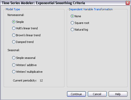
Simple: appropriate for series in which there is no trend or seasonality. | |
|
Holt's linear trend: appropriate for series in which there is a linear trend and no seasonality. | |
|
Brown's linear trend: appropriate for series in which there is a linear trend and no seasonality. | |
|
Damped trend: appropriate for series with a linear trend that is dying out and with no seasonality. | |
|
Simple seasonal: appropriate for series with no trend and a seasonal effect that is constant over time. | |
|
Winters' additive: appropriate for series with a linear trend and a seasonal effect that does not depend on the level of the series. | |
|
Winters' multiplicative: appropriate for series with a linear trend and a seasonal effect that depends on the level of the series. |
Create Models: To use this procedure, starting time and time interval may be defined for the time series. If these have not been defined, click on “Define Dates …” to define starting time and time interval.
Time Series Modeler main dialog box- The procedure allows you to estimate exponential smoothing, univariate or multivariate Autoregressive Integrated Moving Average (ARIMA) model. The procedure can give the best-fitting ARIMA model for one or more dependent variable series. To run Time Series Modeler Procedure, go to Analyze, Time Series, and Create Models. If you already have starting time and time interval (Dates) defined, click OK to open the main dialog box. If you do not need Dates, click OK to open the main dialog box. Among the available tabs under the main dialog box are:
|
Variables- Select one or more dependent variables and one or more independent variables under the “Variables” tab. You can select Expert Modeler, Exponential Smoothing or ARIMA under Method. If you do not want all models, click on Criteria button to make an appropriate selection. Expert Modeler finds the best seasonal or non-seasonal model for a time series. You can limit the search to non-seasonal models. | |
|
Statistics- This allows you to select different goodness of fit measures, statistics for comparing models and statistics for individual models. You can also choose to display forecasts. | |
|
Plots- This allows you to select plots for comparing models or plots for individual models. | |
| Save- This allows you to save some statistics like predicted or residual values. | |
| Options- This allows you to define forecast period. You can set the confidence interval width and specify the maximum number of lags for autocorrelation function output. |
The following movie clip demonstrates how to build an exponential smoothing time series model.
![]() click
here to watch how to create an Exponential Smoothing TS model
click
here to watch how to create an Exponential Smoothing TS model
The data used for this demonstration is Gasoline_Sales data set. See the Data Set page for details. The gasoline sales data is from “An Introduction to Management Science" by Anderson, Sweeney and Williams. The dependent variable is the weekly sales of gasoline in $’000 for twelve week period. We will apply exponential smoothing with a smoothing parameter (or constant) a = 0.2 that was used in the book.
Autoregressive Error Model: This assumes that residuals at times t and t+1 apart are correlated. This model is denoted by AR(1). In general, an autoregressive model of order p, denoted by AR(p), is
where yt = the dependent variables(s) and xt = the independent variable(s).
Moving Average Model: This is like a linear regression model of the current value of the dependent variable (time series) against random shocks of one or more prior values of the time series. In general, a moving average model of order q, denoted by MA(q), is

ARIMA Model: This is a model that combines both the autoregressive and moving average models. A more general model is the Autoregressive Integrated Moving Average (ARIMA) model, which combines the methods of an AR and an MA on a differenced data. This is denoted by ARIMA(p, d, q). In this notation, p = order of autoregressive process, d = order of differencing and q = order of moving average process. If you are not familiar with ARIMA modeling, you should consult textbooks on time series analysis.
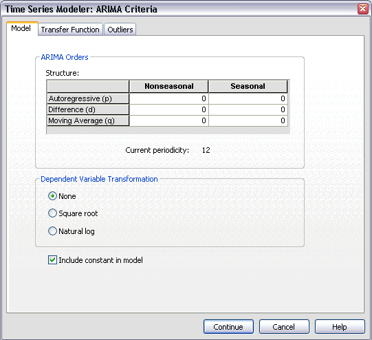
In the following ARIMA criteria dialog box, one needs to specify the order of (p, d, q) for both non-seasonal pattern and seasonal pattern. See SPSS Help Menu for additional information.
|
Autoregressive (p) component: Autoregressive orders specify which previous values from the series are used to predict current values. | |
|
Difference (d) component: Differencing is needed when trends are present and is used to remove their effect. | |
|
Moving Average (q) component:
Moving average orders specify how
deviations from the series mean for previous values are used to predict
current values. |
Expert Time Series Modeler automatically determines the 'best' fit for the time series data. By default, the Expert Modeler considers both exponential smoothing and ARIMA models. User can select only either ARIMA or Smoothing models and specify automatic detection of outliers.
The following movie clip demonstrates how to create an ARIMA model using the ARIMA method and the Expert Modeler provided by SPSS.
![]() click
here to watch how to create an ARIMA model and how to use Expert Molder
click
here to watch how to create an ARIMA model and how to use Expert Molder
The data set used for this demonstration is the Airline_Passenger data set. See the Data Set page for details. The airline passenger data is given as series G in the book Time Series Analysis: Forecasting and Control by Box and Jenkins (1976). The variable 'number' is the monthly passenger totals in thousands. Under the log transformation, the data has been analyzed in the literature.
Apply Time Series Models: This procedure loads an existing time series model from an external file and the model is applied to the active SPSS dataset. This can be used to obtain forecasts for series for which new or revised data are available without starting to build a new model. The main dialog box is similar to the “Create Models” main dialog box.
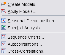
Spectral Analysis: This procedure can be used to show periodic behavior in time series.
Sequence Charts: This procedure is used to plot cases in sequence. To run this procedure, you need a time series data or a dataset that is sorted in certain meaningful order.
Autocorrelations: This procedure plots autocorrelation function and partial autocorrelation function of one or more time series.
Cross-Correlations: This procedure plots the cross-correlation function of two or more time series for positive, negative, and zero lags.
See SPSS Help Menu for additional information on apply time series model, spectral analysis, sequence charts, autocorrelations and cross-correlations procedures.
![]()
![]()
This online SPSS Training Workshop is developed by Dr Carl Lee, Dr Felix Famoye , student assistants Barbara Shelden and Albert Brown , Department of Mathematics, Central Michigan University. All rights reserved.